How to Spot Misleading Graphs in the News

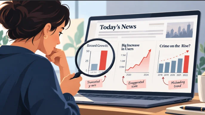
A graph in a news story can make a small change look enormous, turn a temporary fluctuation into an apparent trend, or suggest a relationship the data never established. The numbers may be completely accurate. What misleads you is how they have been selected, scaled and displayed.
Before trusting a chart, look at its axes, time period, units and original source. Then compare the visual impression with the actual figures. Those few checks can reveal whether a dramatic-looking graph tells a dramatic story at all.
A graph can use real numbers and still mislead
Charts work because they let us recognize patterns without reading dozens of numbers. A taller bar suggests more. A rising line suggests growth. A steep downward slope can make a change feel urgent. Those shortcuts are useful, but they also make visual information vulnerable to distortion.
Consider two values: 100 and 105. On a bar chart starting at zero, the second bar is only slightly taller. On a chart whose vertical axis starts at 98, the same five-unit difference can occupy most of the plotting area.
Neither chart has necessarily changed the data. Yet the second creates a much stronger visual impression of growth.
The difference between false data and distorted presentation
There are three distinct problems worth separating:
- Incorrect data: The chart contains values that do not match the underlying evidence.
- Distorted presentation: The values are accurate, but the scale, chart type or visual proportions exaggerate or obscure their meaning.
- Missing context: The chart shows a genuine pattern but excludes information that would materially change how readers interpret it.
Not every misleading graph is deliberately deceptive. Some result from poor design, automatic chart settings or an attempt to simplify complicated information. The reader’s task is to identify what the graph actually establishes, not to guess the designer’s intentions.
Five ways charts can distort the story
Most misleading graphs rely on a fairly small collection of visual choices. Once you recognize them, they become easier to spot in news coverage, advertising, research summaries and social media posts.
A truncated axis makes small changes look dramatic
In a standard bar chart, the height of each bar represents a quantity. If the vertical axis begins above zero, the visible heights no longer reflect the full proportions of the values.
Imagine a report comparing two annual figures, 100 and 105. A chart beginning at 98 makes the second bar appear several times taller than the first, even though the actual increase is just 5%.
The warning sign is a vertical axis that begins close to the lowest value, particularly when the graphic uses filled bars rather than a line. Look at the printed numbers rather than relying on the difference in height.
A non-zero baseline is not automatically dishonest, but it demands attention to what the viewer is supposed to compare.
A narrow time window hides the longer trend
A chart showing only the last two months may accurately depict an increase. It cannot, by itself, establish a sustained upward trend.
Suppose a measure rises from 6.4% to 6.5%. A line connecting those two observations slopes upward. Add earlier months showing that the same measure previously reached 6.9%, and the interpretation changes. The recent increase still happened, but it no longer looks like an uninterrupted climb.
Choosing a limited period is sometimes appropriate. A report about a monthly change needs monthly figures. The problem arises when a short-term movement is presented as evidence of a much larger pattern.
For seasonal measures, such as employment or tourism activity, check whether the figures are seasonally adjusted. Comparing months without accounting for recurring seasonal patterns can introduce another source of confusion.
Unequal scales distort comparisons
Most charts use regularly spaced intervals: 0, 10, 20, 30, and so on. If the distances between labels are inconsistent, equal-looking movements may represent very different numerical changes.
Dual-axis charts require particular care. These display two series against separate vertical scales, often one on each side of the graphic.
For example, a chart could place housing prices on the left axis and interest rates on the right. By adjusting the ranges of those axes, a designer can make the lines appear to rise together or move in opposite directions without changing either dataset.
Two lines crossing also does not establish that the measured quantities are equal. Their positions depend on the chosen scales.
Separate charts using a shared time axis are often clearer when the units differ. If two quantities have the same units, displaying them on one consistent scale usually makes comparison easier.
Percentages hide changes in the underlying totals
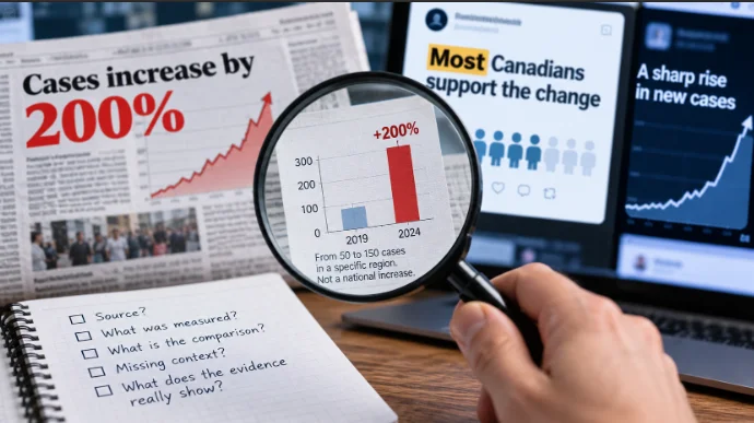
A headline announcing that something has increased by 200% sounds significant. But an increase from two incidents to six is also a 200% rise. The percentage is correct; the absolute numbers tell you how large the change actually is.
Percentages become especially problematic when the denominator changes. A community may record more incidents but a lower rate per 100,000 residents if its population has grown sufficiently.
For any chart showing a percentage increase, ask two questions: What was the starting value, and what total was used to calculate the percentage?
Also distinguish percentage changes from percentage-point changes. A rate rising from 10% to 15% has increased by five percentage points, or 50% relative to its original value. Describing that simply as a 5% increase would be inaccurate.
Three-dimensional graphics exaggerate differences
Three-dimensional bars, tilted pie charts and oversized pictograms can make data harder to compare rather than easier.
Perspective changes the apparent size of objects. A bar positioned at the front may obscure another behind it. In a tilted pie chart, a slice closer to the viewer can appear larger because of its visible area.
Icons introduce a related problem. If an image doubles in both height and width, its area becomes four times larger. A pictogram scaled in two dimensions can therefore make a doubling in the underlying quantity look like a much greater increase.
Simple two-dimensional graphics generally make it easier to compare the actual values. Toronto Metropolitan University’s Critical Data Literacy educational resource illustrates how perspective, selective data and inappropriate chart formats can distort visual information.
When a non-zero baseline is reasonable
The advice to check whether an axis starts at zero is useful, but treating every non-zero axis as misleading goes too far. The right scale depends on the chart’s purpose and the visual property being used to encode the data.
Bar charts and line charts serve different purposes
Bar charts communicate quantities through length. Because the length is measured from a baseline, starting at zero is generally the clearest way to preserve proportional comparisons.
Line charts emphasize positions and changes over time. Their vertical axes do not always need to begin at zero, especially when the purpose is to examine relatively small variations in a measure.
A line chart of temperatures ranging from 18°C to 22°C, for example, may reasonably focus on that interval. Extending the vertical axis down to zero could make meaningful fluctuations almost invisible.
The same logic can apply to unemployment rates, interest rates and other measures that usually occupy a relatively narrow range.
Context determines whether the scale is misleading
A non-zero axis is more defensible when the scale is clearly labelled and the chart is explicitly intended to show small changes rather than relative magnitudes.
Statistics Canada’s Data Visualization: Best Practices, published in February 2023, recommends clear titles, regular intervals and appropriate axis construction, while recognizing exceptions to the general preference for axes beginning at zero.
Rather than applying a universal rule, evaluate whether the design makes the intended comparison understandable.
Here are five illustrative comparisons. The figures are hypothetical examples, not reported research findings.
| Same underlying data | Potentially misleading display | Clearer display |
|---|---|---|
| 100 versus 105 | Bars begin at 98, making the second look several times taller. | Bars begin at zero and show a 5% difference. |
| Rates of 6.9%, 6.4% and 6.5% | Only the last two observations appear, emphasizing a rise. | The earlier observation is included to show the broader movement. |
| Two different quantities over time | Dual axes are adjusted so the lines appear closely related. | Separate charts use clearly labelled, consistent scales. |
| Incidents increase from 2 to 6 | A headline highlights a 200% increase without showing totals. | Both the percentage change and the original counts appear. |
| One quantity is twice another | A pictogram doubles in both height and width, quadrupling its area. | A one-dimensional bar represents the actual two-to-one relationship. |
These examples demonstrate a useful distinction: a chart can highlight a genuine change without necessarily conveying its magnitude fairly.
Rebuild the chart before believing the headline
When a graph makes an important or surprising claim, the most reliable check is to find the original data and compare the visual story with the figures themselves.
A distorted chart is only one part of the problem: spotting misleading statistics also requires checking how the underlying numbers were selected and described.
Find the original table
Consider a real example from Statistics Canada’s Labour Force Survey, September 2026, released on October 9, 2026.
The release reported that the national unemployment rate increased by 0.1 percentage points to 6.5% in September. In British Columbia, the unemployment rate moved in the opposite direction, declining by 0.1 percentage points to 6.4%.
The figures come from Statistics Canada Table 14-10-0287-01, which provides monthly labour force characteristics by geography and other categories.
| Geography | August 2026 | September 2026 | Change |
|---|---|---|---|
| Canada | 6.4% | 6.5% | +0.1 percentage points |
| British Columbia | 6.5% | 6.4% | −0.1 percentage points |
Source: Statistics Canada, Labour Force Survey, September 2026; Table 14-10-0287-01. Rates are seasonally adjusted.
Picture a cropped line chart showing only Canada’s August and September results, with a vertical scale running from 6.35% to 6.55%. The line would climb steeply across most of the available height. A reader might come away with the impression of a major deterioration.
The underlying movement, however, is one-tenth of a percentage point. On its own, the slope says little about the practical size of that change.
Restore the missing context
The same Statistics Canada release provides a longer perspective. Canada’s unemployment rate had reached 6.9% in April 2026 before declining to 6.4% in July and August. September’s rate of 6.5% was also the same as the January rate.
That history does not make the September increase disappear. It establishes that the latest month represented a modest rise within a more varied pattern, not evidence of an uninterrupted increase throughout the year.
The provincial comparison adds another dimension. A national chart cannot tell you whether every province experienced the same movement. British Columbia’s decline demonstrates why the geographic scope of a graph matters.
To check a similar chart yourself:
- Identify the source named beneath the graphic, including any table number or publication date.
- Locate the original dataset and select the same geography, reference period, units and statistical series.
- Compare the plotted values with the source, paying attention to rounding and revisions.
- Extend the time period if the headline makes a broader trend claim.
- Check whether the chart uses seasonally adjusted figures, raw counts, percentages or rates.
For the Labour Force Survey, comparing a seasonally adjusted monthly rate with a different unadjusted series would introduce a new problem rather than resolve the original one.
You do not need specialist software to make a useful comparison. A spreadsheet with a basic line or bar chart can help, provided the dates and values are entered accurately. Sometimes simply reading the source table is enough.
Be careful with downloaded images of charts. A screenshot may remove the footnote explaining a methodological change, a provisional estimate or a revised observation. Check the original publication before treating the image as complete evidence.
A five-second check for any chart in your feed
Most graphs do not require a full investigation. A quick inspection can tell you whether the graphic deserves a closer look before you share it.
- Axis: Does the scale start at zero where proportional comparison requires it? Are the intervals consistent?
- Period: Does the chart show enough time to support the claimed trend?
- Units: Are you looking at counts, percentages, percentage points or rates per population?
- Source: Can you identify the organization and original dataset behind the numbers?
- Headline: Does the wording match the size, direction and scope of the change?
If something feels exaggerated, read the labels before reading the caption again. Check whether the displayed values support the emotional impression created by the design. A dramatic slope may represent a tiny movement, while a visually ordinary chart may contain a genuinely significant change.
The most useful habit is to separate what a graph shows from what its creator wants you to conclude. A good chart makes that distinction easy. A questionable one makes it necessary.